Identification of human control during walking
Jason K. Moore j.k.moore19@csuohio.edu
Sandra K. Hnat
Antonie J. van den Bogert
Human Motion and Control Laboratory [hmc.csuohio.edu]
Cleveland State University
March 4, 2014
Lower Extremity Exoskeletons
Your browser does not support the video tag.
Clips collected from one , two , three , and four .
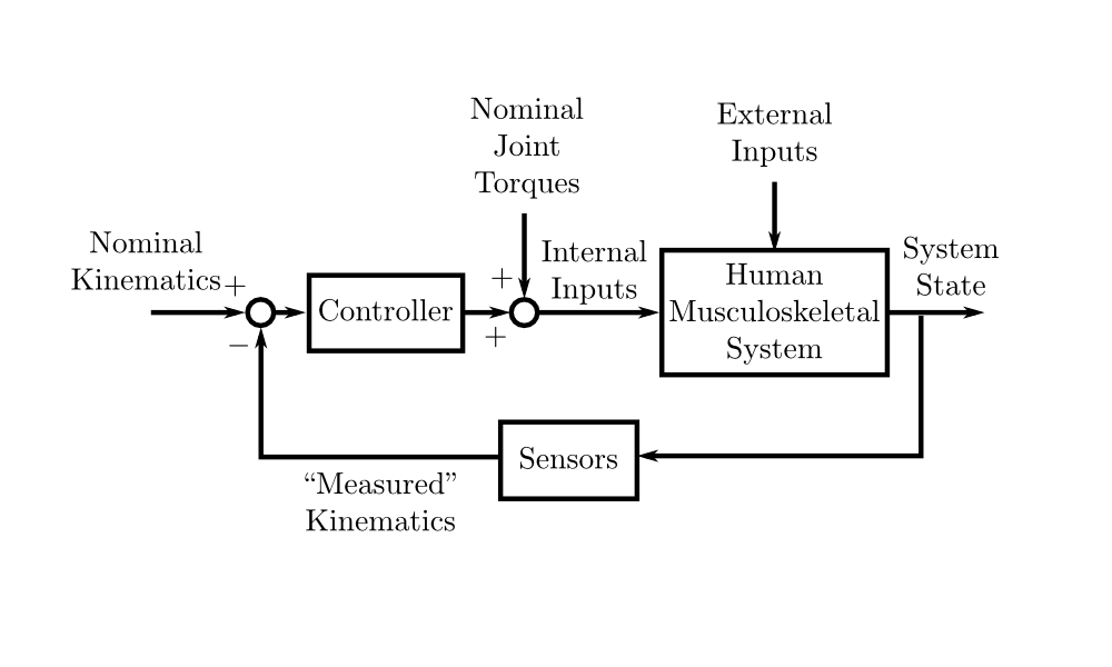
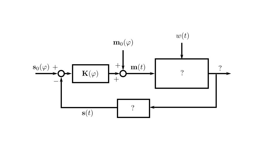
Idealized Gait Feedback Control
Idealized Gait Feedback Control
Estimated
\(\varphi\): Phase of gait cycle
\(\mathbf{s}(\varphi)\): Joint angles and rates
\(\mathbf{m}(\varphi)\): Joint torques
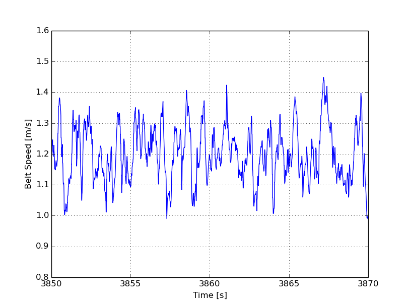
\(w(t)\): Random belt speed
Unknown
\(\mathbf{K}(\varphi)\): Matrix of feedback gains
\(\mathbf{s}_0(\varphi)\): Open loop joint angles and rates
\(\mathbf{m}_0(\varphi)\): Open loop joint torques
Controller Equations
\[
\mathbf{m}(t) = \mathbf{m}_0(\varphi) + \mathbf{K}(\varphi) [\mathbf{s}_0(\varphi) - \mathbf{s}(t)] \\
\]
\[
\mathbf{m}(t) = \mathbf{m}_0(\varphi) + \mathbf{K}(\varphi) \mathbf{s}_0(\varphi) - \mathbf{K}(\varphi) \mathbf{s}(t) \\
\]
Linear Form
\[
\mathbf{m}(t) = \mathbf{m}^*(\varphi) - \mathbf{K}(\varphi) \mathbf{s}(t)
\]
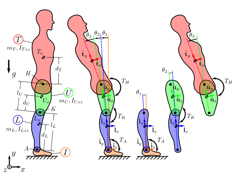
Map Human Control to Exoskeleton
Sensors
Assume that a lower limb exoskeleton can sense relative orientation
and rate of the right and left planar ankle, knee, and hip angles.
\(\mathbf{s}(t) = \begin{bmatrix} s_1 & \dot{s}_1 & \ldots & s_q & \dot{s}_q \end{bmatrix} \) where \(q=6\)
Controls (plant inputs)
Assume that the exoskeleton can generate planar ankle, knee, and hip joint
torques.
\(\mathbf{m}(t) = \begin{bmatrix}m_1 & \ldots & m_q \end{bmatrix} \) where
\(q=6\)
Gain Matrix [Proportional-Derivative Control]
\(
\mathbf{K}(\varphi) =
\begin{bmatrix}
k(\varphi)_{s_1} & k(\varphi)_{\dot{s_1}} & 0 & 0 & 0 & \ldots & 0\\
0 & 0 & k(\varphi)_{s_2} & k(\varphi)_{\dot{s_2}} & 0 & \ldots & \vdots\\
0 & 0 & 0 & 0 & \ddots & 0 & 0\\
0 & 0 & 0 & \ldots & 0 & k(\varphi)_{s_q} & k(\varphi)_{\dot{s}_q} \\
\end{bmatrix}
\)
Linear Least Squares
With \(n\) time samples in each gait cycle and \(m\) steps there are
\(mnq\) equations and which can be used to solve for the \(nq(2q+1)\)
unknowns: \(\mathbf{m}^*(\varphi)\) and \(\mathbf{K}(\varphi)\). This is
a classic overdetermined system of linear equations that can be solved
with linear least squares.
\[\mathbf{A}\mathbf{x}=\mathbf{b}\]
\(\mathbf{A}\): joint angles and rates
\(\mathbf{b}\): joint torques
\(\mathbf{x}\): \(\mathbf{K}\) and \(\mathbf{m}^*\)
\[\mathbf{x}=(\mathbf{A}^T\mathbf{A})^{-1}\mathbf{A}^T\mathbf{b}\]
Experimental Protocol
Full body motion capture: 47 markers
Dual 6 DoF ground reaction forces
8 minutes (500+ steps) of longtidunal perturbations
Three walking speeds: 0.8, 1.2, 1.6 m/s
10+ subjects
Longitudinal perturbations
Random Belt Speed Variations
Random Belt Speed Variations
Your browser does not support the video tag.
Measurement Variations
Measurement Variations
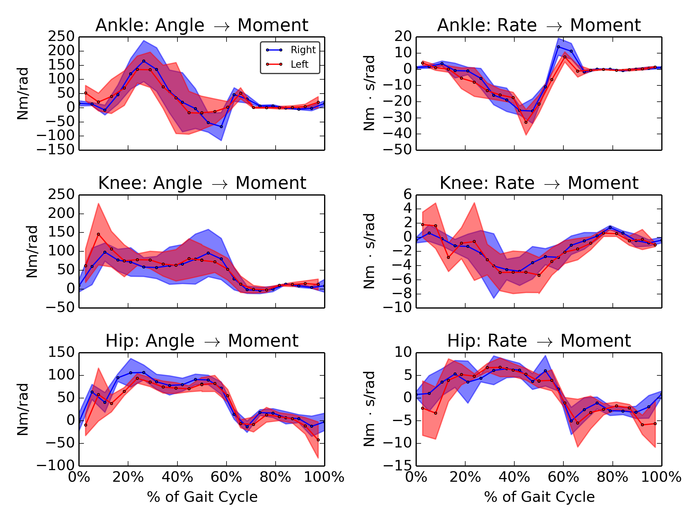
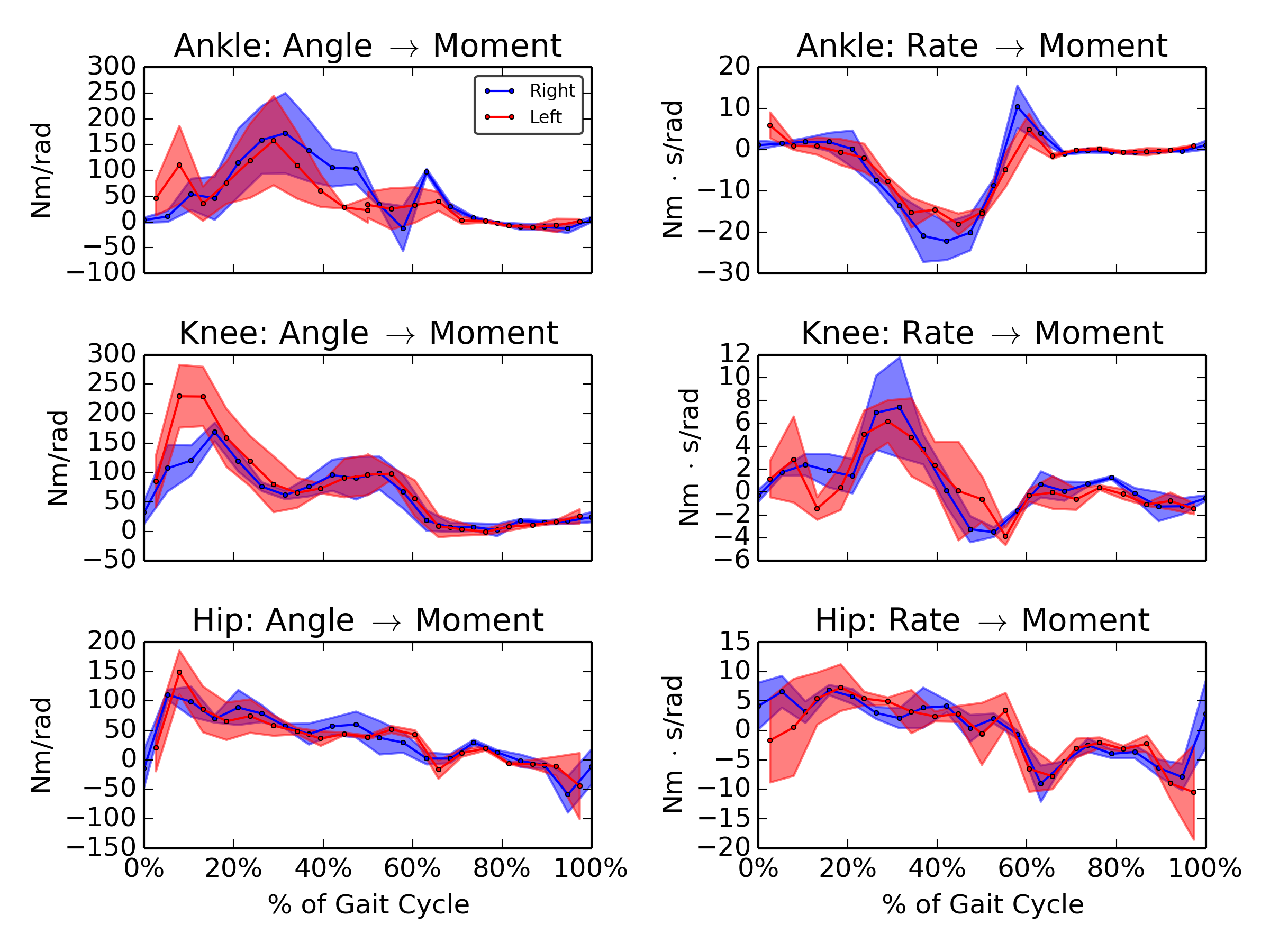
Gains: v=0.8 m/s
Gains: v=1.2 m/s
Gain variation with speed
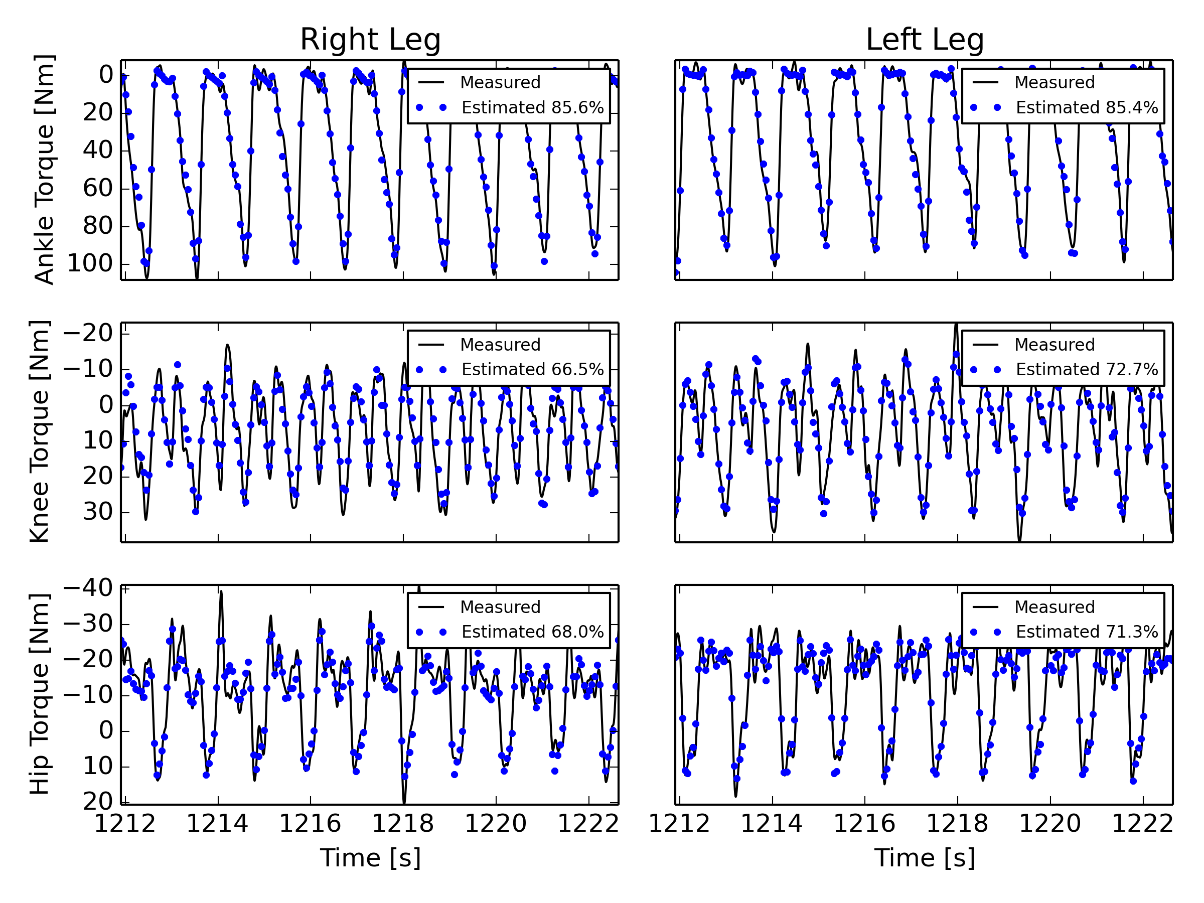
How good is the model?
Summary
Perturbations must be significantly higher that internal system
noise to have any hope of estimating control in this fashion.
Similar gain patterns in each leg.
Similar gain patterns and magnitudes in different subjects.
The model can predict the joint torques for independent data.
Future
Explore full \(\mathbf{K}\) matrix.
Add in time delays.
Remove clock from controller.
Non-linear control models: e.g. neural network.
Use indirect system identification approach with plant model.
Try out the controller on a simulation that has open loop control.
Try out the controller on the Indego exoskeleton.
Information
Contact
Slides
Source code for this analysis
Data