- vr 15 augustus 2014
- misc
- Jason K. Moore
- #ncsrr, #direct collocation, #system identification, #inverted pendulum
This is my last day here at Stanford's Neuromuscular Biomechanics Lab for the NCSRR visiting scholar program. This blog post summarizes what I've done while being here over the last five weeks.
I reviewed the proposal I wrote almost 7 months ago for this visiting position. My main goals were to:
- Implement a closed loop muscle driven gait simulation in Opensim that would simulate significantly faster than the one in [Wang2012] and also include longitudinal and lateral perturbation inputs at the ground surface.
- Run a shooting optimization in the same fashion as [Wang2012] that would discover the control parameters in the closed loop model by minimizing the error in the model's outputs and the gait measurements from subjects being perturbed by walking.
I didn't accomplish either of these goals. During the 6 months between writing the proposal and coming to work here at Stanford Sandy and I collected all of the necessary data and I worked on a computationally simple direct identification technique to identify a control mechanism during walking. The direct identification method "worked" except that I had no way to validate that the gain scheduled controller can actually control something. So an indirect method became more and more appealing than it was when I first wrote the proposal.
I started thinking about the indirect method I'd proposed more deeply and came to realize that the computational costs for the indirect identification technique via shooting that I'd proposed was going to put computation time into number of weeks instead of number of hours, likely regardless of how fast I could make things run. So I started working on understanding the direct collocation techniques that Ton had been using [Ackermann2010] to find optimal open loop control inputs to walking models. This became much more appealing, so over the month before I came out to Stanford I began implementing an identification example for a simpler, known system. I arrived at Stanford with this example close to complete and spent the first couple of weeks getting that to work hoping that it would be suitable for the gait identification problem. It ended up working and seemed promising so I ultimately decided to implement the gait id problem using IPOPT and Opensim. I made strong headway on implementing this but there is still work to be done to see if this method will work on a gait problem. My main accomplishments over the five weeks were:
- Completed a direct collocation identification for a simple inverted pendulum system with promising results.
- Created a joint torque driven planar gait model with prescribed perturbation inputs in Opensim that matches our other Gait2D model implementations.
- Developed a gain scheduled controller that works with the Opensim plant model.
- Developed a skeleton structure for the code to run the direct collocation system id with the closed loop Opensim model. (i.e. idea is in place but implementation still is not complete)
- Learned how to develop with the Opensim API.
- Had lots of fruitful conversations with the other researchers in the NMBL.
Things diverted a bit from my original proposal and I didn't get nearly done the amount I'd proposed. This diversion was the result of finding promising results with the direct collocation approach and finding out that Jack and others had already implemented a 2D gait model which ran even slower than his original 3D model, making shooting based optimization even less appealing.
System Identification with Direct Collocation
System identification is the process of discovering a mathematical model of a dynamic system from measurements of that system. In my case I'm interested in identifying a mathematical model that shows the relationship between what a human senses during walking and the low level actuations of the human's body to produce stable and robust walking using those sensors and actuators that could be realized on an assistive powered prosthetic.
System identification starts with the data. At CSU we've collected typical gait lab data (full body motion capture and ground reaction forces) of several subjects walking for 8 minutes while being longitudinally perturbed with random disturbances at the feet during each stance phase. We believe that this data is rich enough that we can use it to expose a mathematical model of the feedback mechanism used in control during walking.
The objective in system identification is relatively simple. We typically want to minimize the difference in the measurements of a real system and the outputs of a model that represents that system. This is also referred to "tracking" in optimal control jargon. The measurements \(y_m\) are noisy and the model is a mathematical simplification of reality. For discrete measurements, \(y_{mi}\), taken at a sampling interval \(h\) the cost function that needs to be minimized can take this form:
which is an approximation of the continuous form:
\(y\) can be determined by forward simulation of the ODE's that govern the dynamical system given the free system parameters, \(\theta\). But forward simulation of complex dynamical systems, especially stiff ones, can take significant computational time, i.e. often more time than the real motion took. This means that every step in an optimization procedure would have to simulate the system through the entire time period and, for thousands of optimization iterations, this becomes prohibitively computationally expensive. The computational cost is especially high for a system identification problems because they rely on longer measurements to ensure accurate prediction.
But direct collocation formulations and nonlinear programming can potentially speed up the optimization iterations significantly by pushing the evaluation of the equations of motion to nonlinear constraints as opposed to using them for simulation.
A basic nonlinear programming problem with equality constraints then takes this form:
where the cost function, \(J\) is minimized while the free parameters are bounded by \(\theta^L\) and \(\theta^U\) and the equality constraints \(c(\theta)\) are satisfied.
With the cost function specified as shown above, the constraints can be introduced that enforce that \(F=ma\) holds at each collocation node, i.e. \(c(\theta) = F - ma = 0\).
For a typical dynamical system that has a feedback controller that closes the loop, we can describe the system by a set of ordinary differential equations.
First, a structure for the open loop dynamics and the controller are assumed. The open loop dynamics are generally described by a set of ordinary differential equations:
where:
\(x\): system state, depends on time
\(u\): system inputs (composed of those to control and external inputs), depends on time
- \(u^{con}\) : inputs which will be control inputs
- \(u^{ext}\) : disturbance inputs
\(p\): system parameters which are constant with respect to time
\(t\): time
A variety of outputs, \(y\), can be measured from the system. These are generally a function of the state, the inputs, and time, but more likely just a function of state and time.
The simplest controllers that don't introduce any new states to the system can be described as a function of the outputs and new control parameters \(p^{closed}\), often gains. State feedback controllers, as will be used below, fit this model.
State feedback would follow this pattern:
These functions for the controlled inputs can be substituted into the open loop differential equations to get the closed loop dynamics:
These closed loop equations that describe the evolution of the system's states must hold true at any point in time. To transform this continuous equation into a set of constraints for the non-linear programming problem, we first have to make some assumption on the discrete relationship between \(\dot{x}\) and \(f\). There are many different integration approximation methods that could be utilized. Ton has had good luck with backward Euler which is an implicit method and robust for stiff systems. For an integration step size of \(h\), backward Euler integration is:
So \(\dot{x}\) can be approximated by:
or
With this assumption the closed loop equations of motion can be discretized and now fit this form:
So for \(i=1 \ldots N\) collocation nodes, this equation must hold.
The free parameters in the optimization problem always include the state values at the collocation nodes and can include the parameters for the open and closed loop system and the remaining input trajectories (if not known).
For a control parameter identification problem with measured external inputs, \(\theta\) is:
The remaining tricky parts are computing the gradient of the objective function and the Jacobian of the constraints, as these are necessary for the gradient based optimization algorithms employed in NLP solvers.
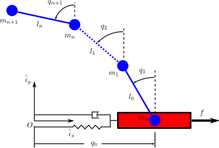
Example Known System: Laterally Perturbed N-Link Pendulum on a Cart
An inverted pendulum is a common system used to model a variety of things about human motion. I decided to start with this simple system to see if the direct collocation method would be successful. The inverted pendulum on a cart is easy to control and the system has well known solutions. The cart with mass \(m_0\) is attached to the origin via a linear spring and damper. It can move laterally along the \(\hat{i}_x\) axis. Attached to the cart are a series of massless links with a mass at each joint. There are actuators at each pin joint that apply a torque between the connected bodies. An external force can be applied to the cart base to perturb the system.
The source code for the following example can be found here:
https://github.com/csu-hmc/inverted-pendulum-sys-id
The first step is to derive the equations for the system. The following gives the open loop equations for a one link system for brevity, but the code supports any number of links:
The states are:
And we will assume the output are simply the coordinates:
Define a state feedback controller symbolically where \(x_{eq} = 0\):
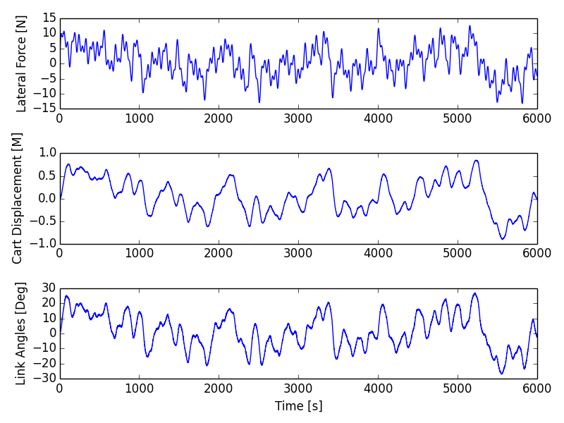
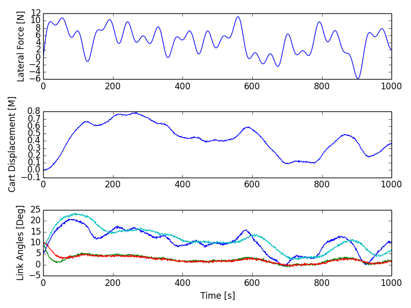
This control law can then be substituted into the open loop equations of motion and the system can be simulated under the influence of cart perturbations (sum of sines):
The numerical values of the controller can easily be found by solving an LQR control problem once the numerical values are chosen for the open loop model parameters. An example simulation is shown below:
The objective function is simply:
where \(y_i\) is a subset of \(\theta\), i.e. just the generalized coordinates. The measurements will have some additive noise:
The gradient of the objective function with respect to \(\theta\) is then:
The closed loop discretized form of the equations of motion look like:
The constraints are evaluated at N-1 collocation nodes (skippin N=1). And given \(\theta\), the ith and (i-1)th states are used along with the controller parameters to compute the right hand side of the system dynamics.
The Jacobian of the constraints is mostly a sparse banded matrix. The parameters, \(k\) don't show up in the kinematic equations so all of those entries are zero. The only other non-zero entries are two values per state for each constraint and values for each dynamic equation constraint (not kinematic) for each of the parameters.
The only partial derivatives we need for evaluating the Jacobian can be found by taking the derivative of \(f_i\) with respect to these variables:
and you get:
These partial derivatives can then be used to build the sparse Jacobian of the constraints. Each row of the constraint Jacobian corresponds to the n state equations at each of the \(N-1\) collocation nodes and the columns correspond to the free parameters, i.e. states at each node and the unknown gains in this case.
I set the rows to follow this convention:
I set the columns to follow this convention:
The sparse entries of the Jacobian can then be computed for each row.
The source code builds functions that evaluates the constraints and the Jacobian of the constraints given \(\theta\) automatically from the symbolic equations of motion. The objective function and gradient are also built, but not yet as automated as the constraints.
To run the pendulum example there is a basic command line interface:
python pendulum.py -h
usage: pendulum.py [-h] [-n NUMLINKS] [-d DURATION] [-s SAMPLERATE]
                   [-i INITIALCONDITIONS] [-r] [-a] [-p]

Run N-Link System ID

optional arguments:
  -h, --help            show this help message and exit
  -n NUMLINKS, --numlinks NUMLINKS
                        The number of links in the pendulum.
  -d DURATION, --duration DURATION
                        The duration of the simulation in seconds.
  -s SAMPLERATE, --samplerate SAMPLERATE
                        The sample rate of the discretization.
  -i INITIALCONDITIONS, --initialconditions INITIALCONDITIONS
                        The type of initial conditions.
  -r, --sensornoise     Add noise to sensor data.
  -a, --animate         Show the pendulum animation.
  -p, --plot            Show result plots.
Running this program does these following steps:
- Constructs the symbolic equations of motion for the open loop system.
- Finds an optimal controller.
- Simulates the closed loop system to generate noisy measurement data.
- Constructs the symbolic closed loop backward Euler discretized constraint equation.
- Constructs the symbolic sparse constraint Jacobian matrix.
- Defines numerical functions that evaluate the objective and it's gradient.
- Defines an IPOPT problem with the above.
- Constructs and initial guess for the solution.
- Runs IPOPT to solve for the free parameters.
- Saves results in a database.
- Makes plots and such.
So for example with a 1 link pendulum (4 unknown gains), a simulation duration of 120 seconds, discretized at 0.01 s (100 Hz), and random initial guess for the gains the problem will be constructed and IPOPT will try to solve it.
The initial guess for the system are the estimated state trajectories and some "close" random values for the gains. The command is:
pendulum.py -n 1 -d 60.0 -r -p -a -s 100.0 -i close
- N = 6,000 (h = 0.01 s (100 hz) over 1 minutes, 60 seconds)
- Number of free variables = 24,008
- Number of non-zero's in the constraint Jacobian = 132,000
IPOPT Results:
197  3.4918824e-03 1.56e-10 7.95e-09 -11.0 1.94e-04    -  1.00e+00 1.00e+00h  1

Number of Iterations....: 197

                                   (scaled)                 (unscaled)
Objective...............:   3.4918824191332988e-03    3.4918824191332988e-03
Dual infeasibility......:   7.9471792187856150e-09    7.9471792187856150e-09
Constraint violation....:   1.4589055009873315e-10    1.5641832273871614e-10
Complementarity.........:   0.0000000000000000e+00    0.0000000000000000e+00
Overall NLP error.......:   7.9471792187856150e-09    7.9471792187856150e-09


Number of objective function evaluations             = 746
Number of objective gradient evaluations             = 198
Number of equality constraint evaluations            = 757
Number of inequality constraint evaluations          = 0
Number of equality constraint Jacobian evaluations   = 198
Number of inequality constraint Jacobian evaluations = 0
Number of Lagrangian Hessian evaluations             = 0
Total CPU secs in IPOPT (w/o function evaluations)   =     94.770
Total CPU secs in NLP function evaluations           =    353.544

EXIT: Optimal Solution Found.
Initial gain guess: [ 107.21621286 14.48140057  37.61288637  -76.37491515]
Known gains:        [  -4.71764346 19.67083668  -3.69402157    5.57114809]
Identified gains:   [  -3.45783597 17.0274554   -3.27007286    5.24318706]
Adding run 36033e34d60ef96463e1b16277e8a4a3fcec9370 to the database.
The total computation time on a laptop PC was ~7.5 minutes. Where as a shooting may have taken 1.5 hours for the same number of iterations and needed a large multi-core machine. This is with a relatively naive implementation and lots of time unnecessary time spent in the function calls.
The constraint violations after finding the optimum look like:
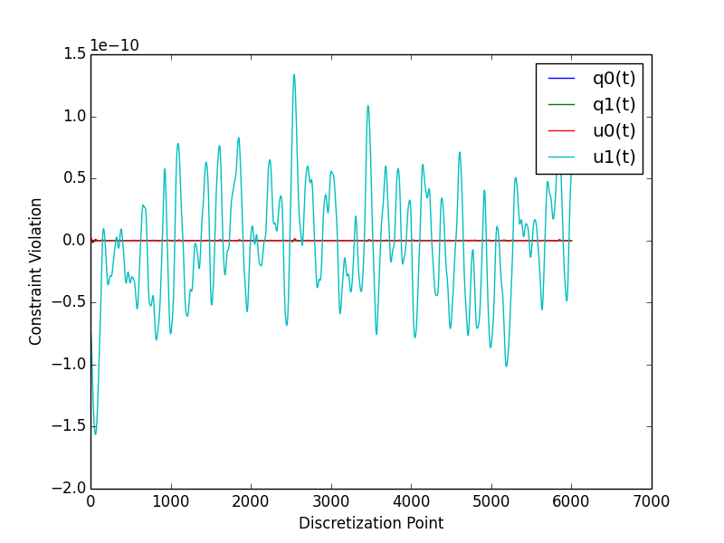
And you can see that the predicted trajectories are tightly aligned with the measurements:
Four Link Pendulum
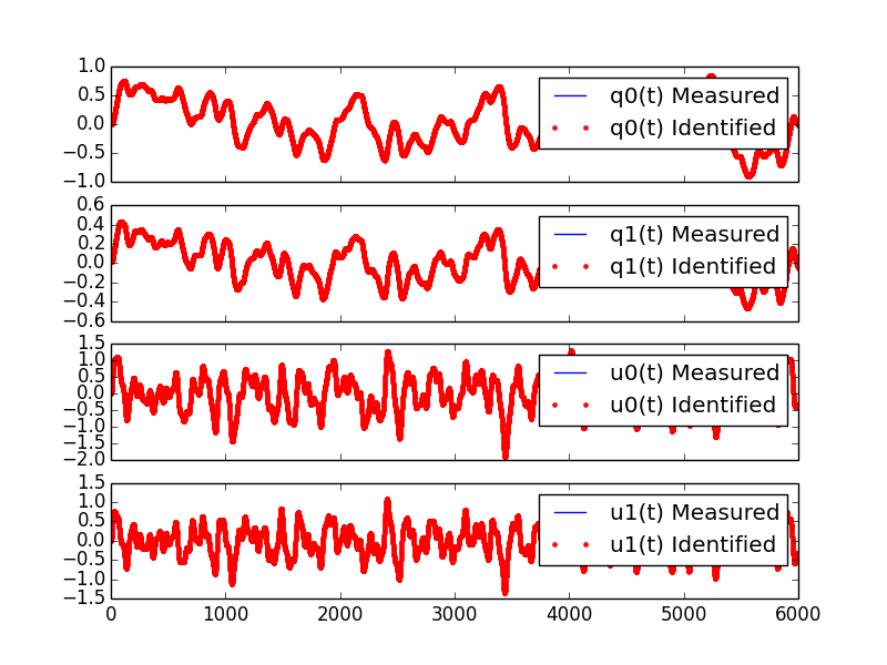
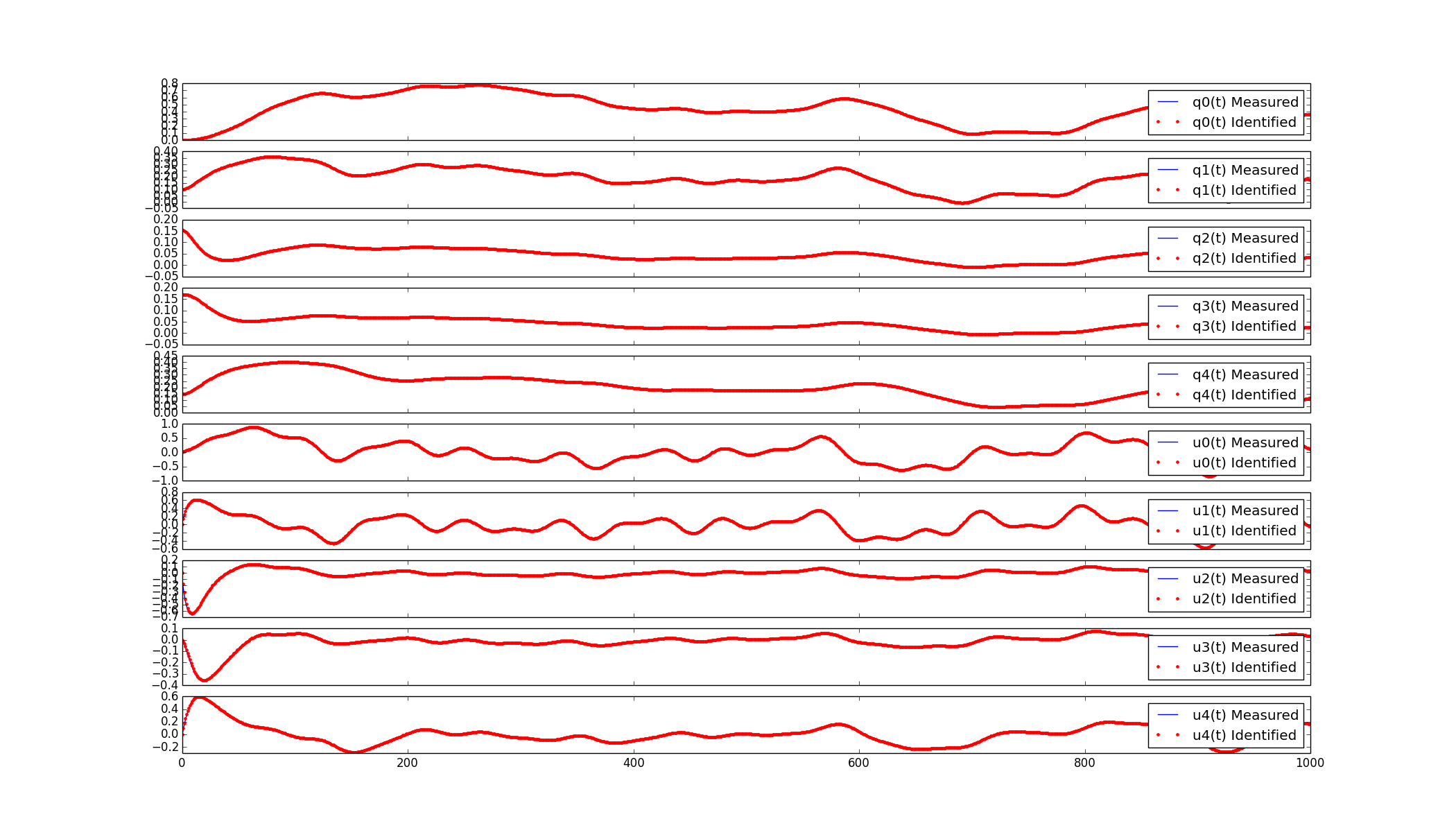
Here are the basic results from four link pendulum solved with very close initial guesses for the 40 gains.
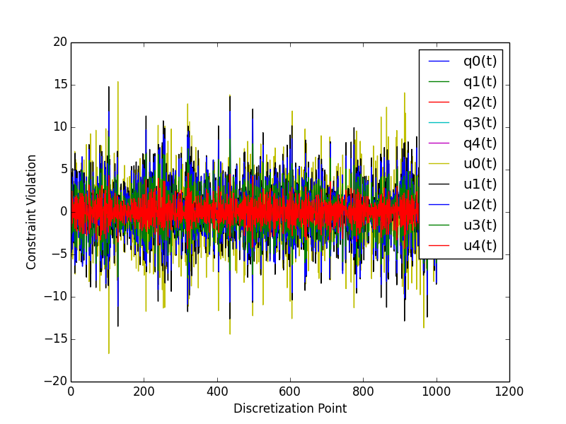
The constraint violations given the known gains:
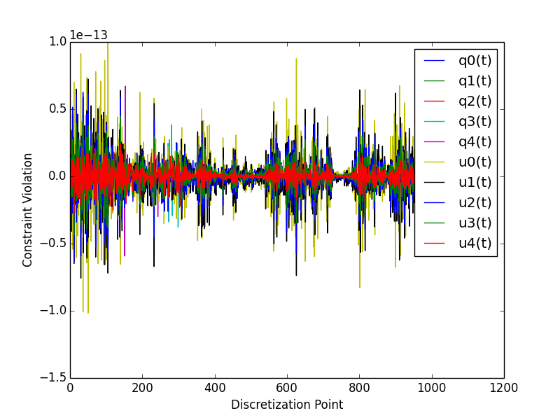
The constraint violations given the optimal gains:
The trajectory comparison:
Planar Gait System ID
Plant
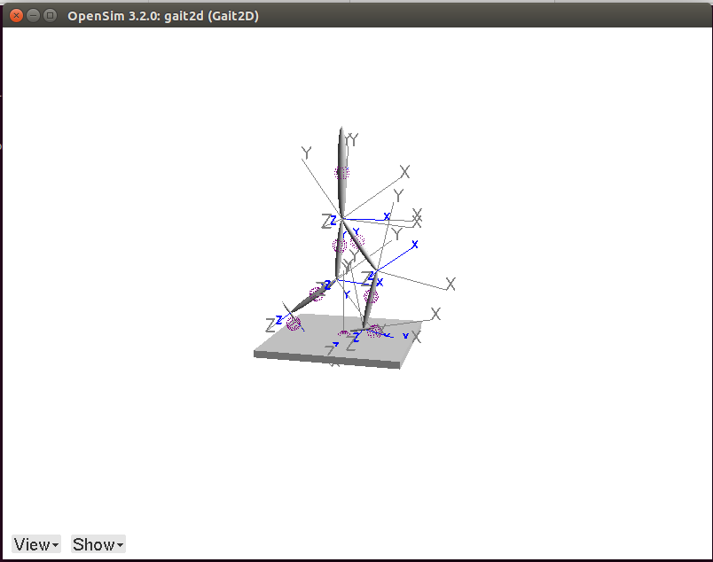
The next step is to implement this for a data collected from perturbed walking. A plant model and controller structure are required. I constructed a planar gait model:
- 7 rigid bodies: trunk, thighs, shanks, feet
- 9 DoF, 18 states
- Compliant heel and toe contact spheres
- Longitudinally translatable floor with prescribed motion input
- Joint torque coordinate actuators: hip, knee, ankle
- Physical parameters from Winters, stored in yaml files
- Still needs subject specific scaling
- Constructed with the Opensim C++ API
Controller
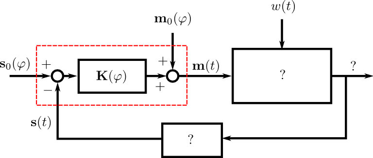
A gain gait cycle scheduled joint angle/rate feedback controller was implemented by sub-classing OpenSim::Controller. It follows this control law:
- \(T\) is the 6 x 1 vector of applied joint torques.
- \(T^*\) is a vector of 6 torques scheduled over the gait cycle at P points.
- \(\mathbf{K}\) is a partial state feedback matrix (6 x 12) scheduled over the gait cycle at P points.
- \(s\) is the 12 x 1 vector of joint angles and angular rates.
The computation uses pre-known heel strike times from the data to compute percent gait cycle for a given time in the simulation. Once the percent gait cycle is known it interpolates from the scheduled \(T^*\) and \(\mathbf{K}\) to get the gains used at the given percentage gait cycle.
Data
The raw data is processed by our gait analysis toolkit. That software outputs csv text files for 8 minute trials sampled at 100 hz that contain columns for:
- ankle, knee, hip joint angles and joint angular rates from inverse kinematics
- spacial trunk location and orientation
- belt position over time
- right and left heelstrike times
These data files are parsed and stored in memory in SimTK::Matrix objects.
The toolkit also computes \(T^*(\varphi)\) and \(\mathbf{K}(\varphi)\) using the direct id method and outputs these to disk. These data files are parsed in C++ to construct std::vectors of SimTK::Vectors/SimTK::Matrices.
Optimize
IPOPT will be used to solve the problem as in the above. It requires a set of information to fully describe the problem.
Variables:
- \(N\) : number of collocation nodes
- \(M\) : number of measured time samples
- \(P\) : Number of gait cycle discretization points
- \(n\) : number of states
- \(o\) : number of model outputs
- \(p\) : total number of model constants
- \(q\) : number of free model constants
- \(r\) : number of free specified inputs
Free parameters:
- \(x\): 18 x N
- \(T^*\): 6 x P
- \(\mathbf{K}\) : 6 x 12 x P
I start by using 3/4 of the data (6 minutes) from each trial for the identification. The remaining 1/4 of data from each trial will be used to validate the identified model. So if If N = 36,000 and n = 18 then the length of \(\theta=648,780\) where there are 780 controller parameters.
The initial guess for the free parameters will be constructed from the estimated state trajectories computed from inverse kinematics and the gains computed from the direct identification approach.
The cost function and it's gradient are defined as they were in the pendulum problem and only the joint coordinates are tracked:
As will the constraints and the Jacobian of the constraints. I will enforce the equation of motion constraints at N - 1 nodes (skip the first node). This is a vector function equal to the number of states:
There are two non zeros per row per state + a nonzero for each free parameter in the dynamic equations (i.e. parameter derivatives are zero in the kinematic equations) giving
The non-zero entries in the Jacobian matrix will be computed via numerical differentiation and stored in a sparse triplet format. So the evaluation of \(c_i\) should be as fast as possible to minimize computation time a this step.
Use IPOPT's limited memory Hessian approximation instead of computing it explicitly.
Solve!
Lessons Learned
The experience at Stanford was very rewarding. Here are some of the highlights:
AOIs were interesting. Each week every person in the lab sends out accomplishments, objectives and issues. The objectives should be concrete goals for the upcoming week. The accomplishments section should list what objectives you completed (and didn't complete) from the previous week. And the issues should detail anything that prevented you from reaching your objectives for that past week. I wasn't using this properly for the first 4 weeks because we weren't given the correct instructions, just told to copy others and it turns out others were not using it correctly either. I've tried this kind of thing for myself in the past, but it has always broken down. In the past, it failed both because there was no one to hold me accountable (I even post them to my lab notebook, but no one actually reads that) and I didn't always write down concrete goals that were within a week's scope.
The AOIs are, in general, a good idea. But there are some things I'd do differently.
People rarely use the issues. My hunch is that, in a group, people want to seem like they are accomplishing a lot and have little trouble doing so. That could be especially true in a place like Stanford. I have a feeling that there are more issues in the week that aren't shown. I think this is typical in science in general. We show our best results in the paper, i.e. the results that we just barely got to work, yet don't show the faults of the method or the difficulties. I wonder if naming this section something different could help people be more willing to share their issues. It may be nice to come up with a word that invokes a positiveness to the topic "Looking back on the week, what would have helped you meet you objectives?", or "What would have helped you meet your objectives faster?", or "What information/knowledge/etc is needed to make a big stride towards your objective?", "What during the past week came up that you wish you had a teammate to collectively solve the problem with?".
I felt the need to write a lot in my accomplishments so that I didn't look like I'm doing less than other people (which I generally felt). Competition is probably good, it helps me improve my performance and be more efficient but it can also be a drain. Others may not feel like the accomplishments are competitive but it may be good to think about how to make it feel like a healthy competition. I'm at the point in my career where I'm finally getting tired of working late into the night and 60+ hours a week and I often choose to sleep or not work to keep those hours of work more sane. This article made me think about being more real with myself about the # of hours I want to work:
It was refreshing to be in an environment where lots of people can help answer questions that you have. The lab was structured with quite a few "permanent" PhD level researchers that essentially ran the Opensim project and assisted students in their research objectives. This was infinitely better than it is at CSU where I seem to be the only post doc in existence. Everyone seemed to collaborate pretty well too. One student said he didn't think anyone actually collaborated on individual research projects, but there was solid collaboration on the Opensim development and they'd just started really utilizing Github with PR's and issues. I suspect research labs could be much more efficient if they could support a fair number of permanent high level researcher positions. But things were still centered around very individual research projects for each student.
Ok, closing this one off. It's already too long. Thanks for the opportunity to hang out and work in the NMBL!
References
| [Wang2012] | (1, 2) Wang, Jack M., Samuel R. Hamner, Scott L. Delp, and Vladlen Koltun. “Optimizing Locomotion Controllers Using Biologically-Based Actuators and Objectives.” ACM Transactions on Graphics (TOG) 31, no. 4 (2012): 25. |
| [Ackermann2010] | Ackermann, Marko, and Antonie J. van den Bogert. “Optimality Principles for Model-Based Prediction of Human Gait.” Journal of Biomechanics 43, no. 6 (April 19, 2010): 1055–60. doi:10.1016/j.jbiomech.2009.12.012. |
Notes
These are just some notes I took from the comments after I presented this:
- Look up OpenMP for parallel stuff.
- Mombaur, Katja Daniela supposedly does open loop direct collocation for walking.
- Parallelize the jacobian evaluation because you only need certain parameters for each row in the jacobian.
- Think about using different integrator assumptions so you can increase h.
- Add the plant controller diagram before the system id explanation.
- Boyd Convex Optimization
Constrained multibody dynamics problems:
Basic form with lagrange multipliers:
M u' = f - G^T lam Gu' = 0
G u' + G M^-1 G^T lam = G M^-1 f G M^-1 G^T lam = G M^-1 f
G M^-1 G^T lam = u_o