- wo 23 april 2014
- notebook
- Jason K. Moore
- #notebook, #gait, #system identification, #control
This is potentially a very simple way to think about what we measure and estimate from force plate and motion capture data during gait and how it connects to the active forces we generate from our muscles for control. To avoid non-linearities and keep things simple here is a three particle model:
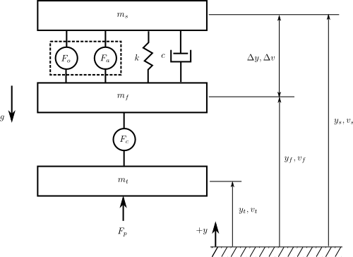
- \(m_t\): the treadmill mass
- \(m_f\): the foot mass
- \(m_s\): the shank mass
- \(F_p\): the force applied to perturb the displacement of the treadmill, and thus the whole system
- \(F_c\): the contact force between the foot at the treadmill. There are models that can represent contact, but for now I'll just assume that it is some kind of force producer. [1]
- \(F_0\), \(F_a\): Both of these are active forces applied between the foot and the shank. This is synonymous to the forces generated by actively controlling the muscles that connect the two bodies and can be generalized to joint torques for a typical walking model. The reason for having two will be explained below.
- \(k\), \(c\): Coefficients for simple linear stiffness and damping force generators that represent the passive portions force generators between the foot and the shank.
- \(y_t,y_f,y_s\): The distances of each mass above the ground.
- \(\Delta y\): The distance between the foot and shank, synonymous with a joint angle.
The equations of motion of this system look like this:
Since I define \(F_c\) as a generic force, the top equation is not coupled to the bottom two. Now thinking about the second equation, I can measure, or estimate reasonably well, these quantities: \(\Delta y, g, m_f, \dot{v}_f, F_c\). So inverse dynamics says we can solve for \(F\) given our measurements:
\(F\) is synonymous with the joint torques that we estimate from inverse dynamics in a typical gait analysis. But \(F\) is also the sum of both the passive and active forces in the joint.
So if we can estimate \(F\) with inverse dynamics then all I need are reasonable estimates of the passive portion of the joint forces, i.e. \(c\) and \(k\) in this case to compute the active forces.
Now if there is a real system that can be reasonably modeled by the above I could excite it, cause some motion, take the measurements, and compute an estimate of the total force acting between the foot and shank, i.e. \(F\).
At this point I can define what the active forces, \(F_a,F_0\) are. Gait is periodic, so if \(F_p=0\), :math`F_a=0`, and \(F_0=sin(t)\) are used to excite the real system, there will be some steady state periodic motion of the system. We call the steady state of \(\Delta y\) and \(\Delta v\) \(y_0\) and \(v_0\), respectively. These two are synonymous with the "open loop" joint angles and rates that can drive a gait model for walking. This steady state can be thought of as the desired system state, i.e. the state trajectories we want to track while the system is being perturbed.
So now if I perturb this oscillating real system with \(F_p\neq0\), white noise for example, then then \(\Delta y\) and \(\Delta v\) will no longer equal \(y_0\) and \(v_0\). We can then think of \(F_a\) as a force that applies some feedback to drive \(\Delta y,\Delta v\) to \(y_0,v_0\). This can be written as so:
The equation for the joint forces then become:
I can measure or estimate only \(F\), \(\Delta v\), and \(\Delta y\). The ideal goal is to figure out what \(c_a\) and \(k_a\) are, i.e. the active gains in the controller. If \(F_0\) and \(v_0\) are periodic and I have enough measurements in time, i.e. from multiple periods, then I can get estimates of \(c_t=c-c_a\) and \(k_t=k-k_a\). These are the combined passive and active stiffness and damping coefficients. This formulation will also allow the estimation of this periodic term:
This shows that the best I can do is to estimate "gains" which are combinations of the stiffness and damping from passive and active forces.
But if I collect data when \(F_p=0\) we can possibly get estimates of \(v_0\) and \(y_0\) which could allow me to estimate both the active and passive gains, independently.
Other researchers in biomechanics talk about "impedance" and "joint impedance". For example in [Rouse2012] defines impedance in the ankle joint as:
\(T_i\) is the "joint torque" but he doesn't use standard inverse dynamics, he neglects the foot mass, so his joint torque estimate is basically the measured ground reaction moment. It follows this form:
Now if \(T_a\) is a PD controller, as described above, you get:
and then:
In his experiments, he collects data during the stance phase for one foot over and over again (something like 400 steps per subject) with one of four perturbations applied during each step. He measures or estimates the "joint torque" [2], \(T_i\), and the ankle angle, \(\theta\) (\(\ddot{\theta}\) and \(\dot{\theta}\) are computed by numerical differentiation). A simple linear least squares is then used to estimate \(I_i,c_i\), and \(k_i\). He assumes that these parameters are time invariant (at least for the stance phase).
If we compare his "impedance" model to my formulation we see:
So his estimated parameters are not only a lumping of active and passive torque coefficients, but also gravitational terms. And he completely neglects the terms I call \(F^*\) above (here we can use \(T^*\) for the last equations). But he is able to find impedance parameters such that his model fits the data he collected, even when neglecting this constant term. It likely gets lumped into the output error of the linear least squares fit and may be small.
| [Rouse2012] | Rouse et al., “Estimation of Human Ankle Impedance during Walking Using the Perturberator Robot.” |
| [1] | Note that this ignores the fact that forces plates measure the forces between two masses. Inertial effects has to be accounted for when moving the force plate, but the following analysis assumes we can measure the force at the surface (not at the load cells). |
| [2] | This is not the traditional joint torque because it includes inertial and gravitational effects in addition to passive and active joint torques. |